
Deep learning for NeuroImaging in Python.
Note
Go to the end to download the full example code.
UNet segmentation
Credit: A Grigis
A simple example on how to use the SphericalUNet architecture on the classification dataset.
import numpy as np
import matplotlib.pyplot as plt
import torch
from torch import nn
from torch.utils.data import DataLoader
from surfify import utils
from surfify import plotting
from surfify import models
from surfify import datasets
Inspect dataset
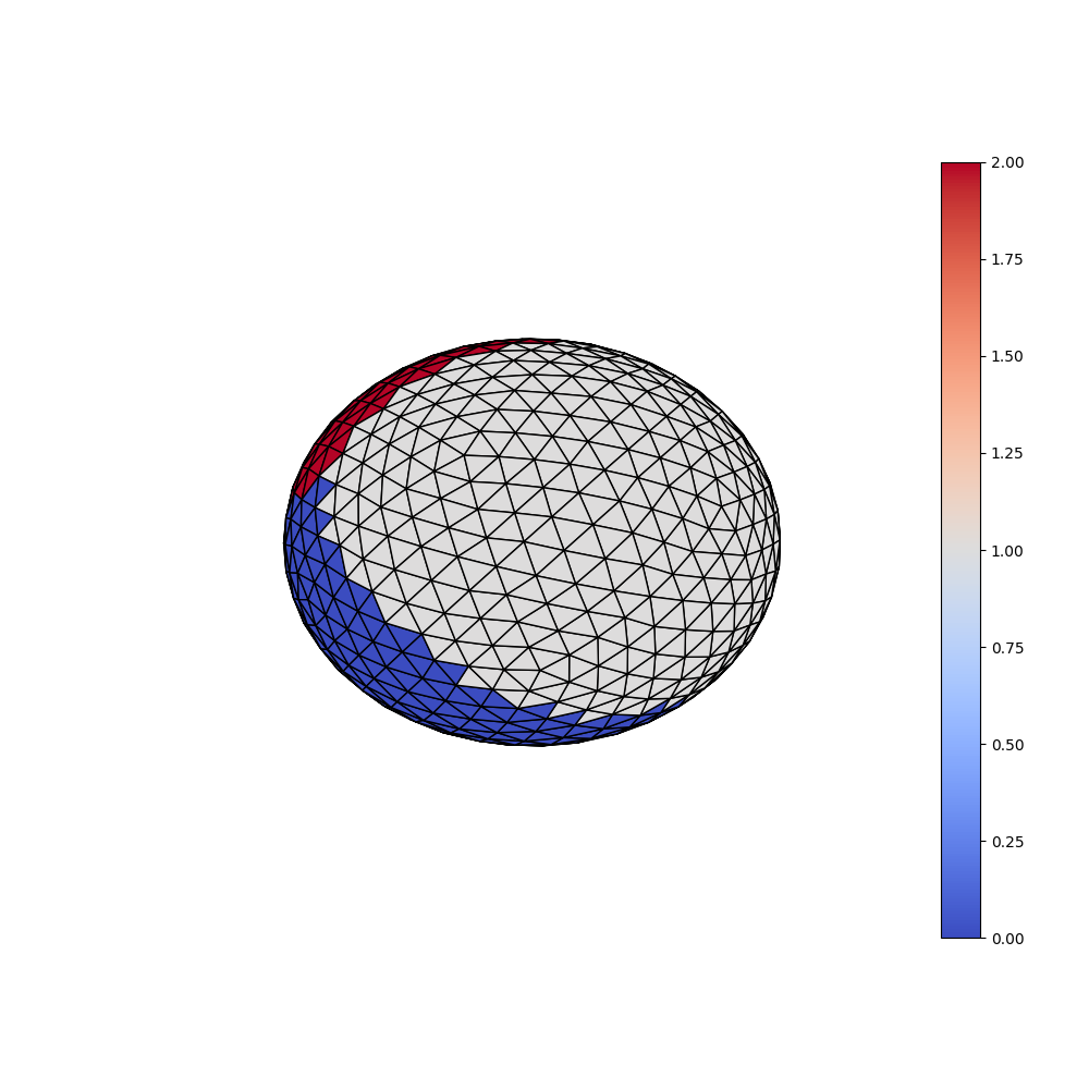
First we load the classification dataset (with 3 classes) and inspect the genrated labels.
standard_ico = True
ico_order = 3
n_classes = 3
n_epochs = 20
ico_vertices, ico_triangles = utils.icosahedron(
    order=ico_order, standard_ico=standard_ico)
n_vertices = len(ico_vertices)
X, y = datasets.make_classification(
    ico_vertices, n_samples=40, n_classes=n_classes, scale=1, seed=42)
print("Surface:", ico_vertices.shape, ico_triangles.shape)
print("Data:", X.shape, y.shape)
plotting.plot_trisurf(ico_vertices, ico_triangles, y, is_label=True)

Surface: (642, 3) (1280, 3)
Data: (40, 3, 642) (642,)
Train the model
We now train the SphericalUNet model using a CrossEntropy loss and a SGD optimizer. As it is obvious to segment the input classification dataset an accuracy of 100% is expected.
dataset = datasets.ClassificationDataset(
    ico_vertices, n_samples=40, n_classes=n_classes, scale=1, seed=42)
loader = DataLoader(dataset, batch_size=5, shuffle=True)
model = models.SphericalUNet(
    in_order=ico_order, in_channels=n_classes, out_channels=n_classes,
    depth=2, start_filts=8, conv_mode="DiNe", dine_size=1, up_mode="transpose",
    standard_ico=standard_ico)
loss_fn = nn.CrossEntropyLoss()
optimizer = torch.optim.SGD(
    model.parameters(), lr=0.1, momentum=0.99, weight_decay=1e-4)
size = len(loader.dataset)
n_batches = len(loader)
for epoch in range(n_epochs):
    for batch, (X, y) in enumerate(loader):
        pred = model(X)
        loss = loss_fn(pred, y)
        optimizer.zero_grad()
        loss.backward()
        optimizer.step()
        loss, current = loss.item(), batch * len(X)
        if epoch % 5 == 0:
            print("loss {0}: {1:>7f}  [{2:>5d}/{3:>5d}]".format(
                epoch, loss, current, size))
model.eval()
test_loss, correct = 0, 0
y_preds = []
with torch.no_grad():
    for X, y in loader:
        pred = model(X)
        test_loss += loss_fn(pred, y).item()
        logit = torch.nn.functional.softmax(pred, dim=1)
        y_pred = pred.argmax(dim=1)
        correct += (y_pred == y).type(torch.float).sum().item()
        y_preds.append(y_pred.numpy())
test_loss /= n_batches
correct /= (size * n_vertices)
y_preds = np.concatenate(y_preds, axis=0)
print("Test Error: \n Accuracy: {0:>0.1f}%, Avg loss: {1:>8f}".format(
    100 * correct, test_loss))
loss 0: 1.187070  [    0/   40]
loss 0: 0.979653  [    5/   40]
loss 0: 0.855242  [   10/   40]
loss 0: 0.712914  [   15/   40]
loss 0: 0.607041  [   20/   40]
loss 0: 0.516769  [   25/   40]
loss 0: 0.425260  [   30/   40]
loss 0: 0.333251  [   35/   40]
loss 5: 0.001165  [    0/   40]
loss 5: 0.001057  [    5/   40]
loss 5: 0.001287  [   10/   40]
loss 5: 0.001859  [   15/   40]
loss 5: 0.002577  [   20/   40]
loss 5: 0.002806  [   25/   40]
loss 5: 0.002196  [   30/   40]
loss 5: 0.001267  [   35/   40]
loss 10: 0.000006  [    0/   40]
loss 10: 0.000006  [    5/   40]
loss 10: 0.000005  [   10/   40]
loss 10: 0.000005  [   15/   40]
loss 10: 0.000006  [   20/   40]
loss 10: 0.000006  [   25/   40]
loss 10: 0.000007  [   30/   40]
loss 10: 0.000009  [   35/   40]
loss 15: 0.000006  [    0/   40]
loss 15: 0.000006  [    5/   40]
loss 15: 0.000007  [   10/   40]
loss 15: 0.000009  [   15/   40]
loss 15: 0.000010  [   20/   40]
loss 15: 0.000011  [   25/   40]
loss 15: 0.000013  [   30/   40]
loss 15: 0.000014  [   35/   40]
Test Error:
 Accuracy: 100.0%, Avg loss: 0.000001
Inspect the predicted labels
Finally the predicted labels of the first sample are displayed. As expected they corresspond exactly to the ground truth.
plotting.plot_trisurf(ico_vertices, ico_triangles, y_preds[0], is_label=True)
plt.show()
Total running time of the script: (0 minutes 5.727 seconds)
Estimated memory usage: 565 MB
Follow us