
Deep learning for NeuroImaging in Python.
Note
This page is a reference documentation. It only explains the class signature, and not how to use it. Please refer to the gallery for the big picture.
- class nidl.losses.yaware_infonce.KernelMetric(kernel='gaussian', bandwidth: str | float | list[float] | ndarray = 'scott')[source]
Bases:
BaseEstimatorInterface for fast weighting matrix computation.
It computes a weighting matrix
 between input samples based on
Kernel Density Estimation (KDE) [R30], [R31]. Concretely, it computes the
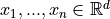
following weighting matrix between multivariate samples
between input samples based on
Kernel Density Estimation (KDE) [R30], [R31]. Concretely, it computes the
following weighting matrix between multivariate samples
 :
: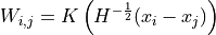
with
 a kernel (or “weighting function”) such that:
 (positive)
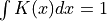 (normalized)
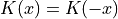 (symmetric)
and
 is the bandwidth in the KDE
estimation of p(X).
is the bandwidth in the KDE
estimation of p(X). is a symmetric definite-positive and it can be automatically
computed based on Scott’s rule [R32] or Silverman’s rule [R33] if required.
In that case, the bandwidth is computed as a scaled version of the
diagonal terms in the data covariance matrix:
is a symmetric definite-positive and it can be automatically
computed based on Scott’s rule [R32] or Silverman’s rule [R33] if required.
In that case, the bandwidth is computed as a scaled version of the
diagonal terms in the data covariance matrix:
- Parameters:
kernel : {‘gaussian’, ‘epanechnikov’, ‘exponential’, ‘linear’, ‘cosine’}, default=’gaussian’
The kernel applied to the distance between samples.
bandwidth : {‘scott’, ‘silverman’} or float or list of float, default=”scott”
The method used to calculate the estimator bandwidth:
If bandwidth is ‘scott’ or ‘silverman’,
is a scaled
version of the diagonal terms in the data covariance matrix.If bandwidth is scalar (float or int),
is set to a
diagonal matrix:
![H = \mathrm{diag}([bandwidth,\ldots, bandwidth])](../_images/math/2a4e0f928998e9d1b8a55411ccfb5e39db5c2e88.png) .
.If bandwidth is a list of floats,
is a diagonal matrix
with the list values on the diagonal:
 .
.If bandwidth is a 2d array, it must be of shape (n_features, n_features)
Notes
Scott’s Rule [R30] estimates the bandwidth as:
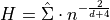
where
 is the covariance matrix of the data,
 is the number of samples, and
  is the number of
features (
is the number of
features ( for univariate data). Here, we only consider
the diagonal terms (assuming features decorrelation) for numerical
stability.
for univariate data). Here, we only consider
the diagonal terms (assuming features decorrelation) for numerical
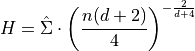
stability.Silverman’s rule of thumb [R31] for multivariate data is:
References
[R30] (1,2,3)Rosenblatt, M. (1956). “Remarks on some nonparametric estimates of a density function”. Annals of Mathematical Statistics.
[R31] (1,2,3)Parzen, E. (1962). “On estimation of a probability density function and mode”. Annals of Mathematicals Statistics.
- fit(X)[source]
Computes the bandwidth in the kernel density estimation.
- Parameters:
X : array of shape (n_samples, n_features)
Input data used to estimate the bandwidth (based on covariance matrix).
- Returns:
self : KernelMetric
- pairwise(X)[source]
- Parameters:
X : array of shape (n_samples, n_features)
Input data.
- Returns:
S : array of shape (n_samples, n_samples)
Similarity matrix between input data.
Follow us