Note
Go to the end to download the full example code.
Self-Supervised Learning with Barlow Twins
This tutorial will show you how to fit and evaluate a Barlow Twins model [1] on the OpenBHB dataset using NIDL.
We will follow these steps using the NIDL library:
Load the OpenBHB dataset.
Define the data augmentations for self-supervised training.
Define the BarlowTwins model.
Train the model.
Visualize the model’s embedding using MDS and evaluate its performance on age prediction using linear regression and KNN.
As for the neuroimaging data, we will investigate two input representations:
Voxel-based morphometry (VBM) maps, which are preprocessed gray matter density maps.
Surface-based morphometry (SBM) maps, which are cortical thickness, mean curvature, gray matter volume and surface area maps projected onto a standard surface template.
Both representations are available in the OpenBHB dataset. To make the training faster and reduce the memory footprint, we will consider regions of interest (ROIs) instead of the whole brain. For VBM, we will use the mean gray matter density averaged within each ROI of the Neuromorphometrics atlas (284 regions). For SBM, we will use the cortical thickness, mean curvature, gray matter volume and surface area averaged within each ROI of the Desikan-Killiany atlas (68 regions).
The Barlow Twins model will be trained individually on both representations and we will compare their performance on age prediction.
Setup
This notebook requires some packages besides nidl. Let’s first start with importing our standard libraries below:
import matplotlib.pyplot as plt
import numpy as np
import torchvision.transforms as transforms
from sklearn.linear_model import LinearRegression
from sklearn.manifold import MDS
from sklearn.metrics import mean_absolute_error, r2_score
from sklearn.neighbors import KNeighborsRegressor
from torch.utils.data import DataLoader
from torchvision.ops import MLP

from nidl.datasets import OpenBHB
from nidl.estimators.ssl import BarlowTwins
from nidl.transforms.transforms import MultiViewsTransform
We define some global parameters that will be used throughout the notebook:
data_dir = "/tmp/openBHB"
batch_size = 128
num_workers = 10
latent_size = 32
OpenBHB datasets and data augmentations for Barlow Twins training
We will use the OpenBHB dataset for pre-training the models. We will focus on the VBM ROI representation and the SBM ROI representation for this tutorial. Since they are tabular data, we will use random masking and adding Gaussian noise as data augmentation in contrastive learning.
# Hyperparameters for data augmentations
mask_prob = 0.8
noise_std = 0.5
contrast_transforms = transforms.Compose(
    [
        lambda x: x.flatten(),
        lambda x: (np.random.rand(*x.shape) > mask_prob).astype(np.float32)
        * x,  # random masking
        lambda x: x
        + (
            (np.random.rand() > 0.5) * np.random.randn(*x.shape) * noise_std
        ).astype(np.float32),  # random Gaussian noise
    ]
)
We first create the SSL dataloaders with VBM modality and age as weak label. We use the previous contrastive transforms for data augmentation.
dataloader_ssl_vbm = DataLoader(
    OpenBHB(
        data_dir,
        modality="vbm_roi",
        target=None,
        transforms=MultiViewsTransform(contrast_transforms, n_views=2),
        streaming=False,
    ),
    batch_size=batch_size,
    num_workers=num_workers,
    shuffle=True,
)
dataloader_ssl_vbm_test = DataLoader(
    OpenBHB(
        data_dir,
        modality="vbm_roi",
        target=None,
        split="val",
        transforms=MultiViewsTransform(contrast_transforms, n_views=2),
        streaming=False,
    ),
    batch_size=batch_size,
    num_workers=num_workers,
    shuffle=False,
)
/opt/hostedtoolcache/Python/3.12.13/x64/lib/python3.12/site-packages/torch/utils/data/dataloader.py:424: UserWarning: This DataLoader will create 10 worker processes in total. Our suggested max number of worker in current system is 4, which is smaller than what this DataLoader is going to create. Please be aware that excessive worker creation might get DataLoader running slow or even freeze, lower the worker number to avoid potential slowness/freeze if necessary.
  self.check_worker_number_rationality()
Then, we create the SSL dataloaders with SBM modality on the Desikan-Killiany atlas and age as weak label. We only extract some surface features and we use the same contrastive transforms as for VBM.
# Extract only surface area, GM volume, cortical thickness, mean curvature for
# SBM maps
sbm_channels = [0, 1, 2, 5]


def sbm_transform(x):
    return x[sbm_channels].flatten()


def vbm_transform(x):
    return x.flatten()


dataloader_ssl_sbm = DataLoader(
    OpenBHB(
        data_dir,
        modality="fs_desikan_roi",
        target=None,
        transforms=MultiViewsTransform(
            transforms.Compose([sbm_transform, contrast_transforms]), n_views=2
        ),
        streaming=False,
    ),
    batch_size=batch_size,
    num_workers=num_workers,
    shuffle=True,
)
dataloader_ssl_sbm_test = DataLoader(
    OpenBHB(
        data_dir,
        modality="fs_desikan_roi",
        target=None,
        split="val",
        transforms=MultiViewsTransform(
            transforms.Compose([sbm_transform, contrast_transforms]), n_views=2
        ),
        streaming=False,
    ),
    batch_size=batch_size,
    num_workers=num_workers,
    shuffle=False,
)
/opt/hostedtoolcache/Python/3.12.13/x64/lib/python3.12/site-packages/torch/utils/data/dataloader.py:424: UserWarning: This DataLoader will create 10 worker processes in total. Our suggested max number of worker in current system is 4, which is smaller than what this DataLoader is going to create. Please be aware that excessive worker creation might get DataLoader running slow or even freeze, lower the worker number to avoid potential slowness/freeze if necessary.
  self.check_worker_number_rationality()
/opt/hostedtoolcache/Python/3.12.13/x64/lib/python3.12/site-packages/torch/utils/data/dataloader.py:424: UserWarning: This DataLoader will create 10 worker processes in total. Our suggested max number of worker in current system is 4, which is smaller than what this DataLoader is going to create. Please be aware that excessive worker creation might get DataLoader running slow or even freeze, lower the worker number to avoid potential slowness/freeze if necessary.
  self.check_worker_number_rationality()
Finally, we create the dataloaders for evaluating the learned representations on age prediction. We don’t apply any data augmentation here.
dataloader_vbm_train = DataLoader(
    OpenBHB(
        data_dir,
        modality="vbm_roi",
        target="age",
        split="train",
        transforms=vbm_transform,
        streaming=False,
    ),
    batch_size=batch_size,
    num_workers=num_workers,
    shuffle=False,
)

dataloader_vbm_test = DataLoader(
    OpenBHB(
        data_dir,
        modality="vbm_roi",
        target="age",
        split="val",
        transforms=vbm_transform,
        streaming=False,
    ),
    batch_size=batch_size,
    num_workers=num_workers,
    shuffle=False,
)

dataloader_sbm_train = DataLoader(
    OpenBHB(
        data_dir,
        modality="fs_desikan_roi",
        target="age",
        split="train",
        transforms=sbm_transform,
        streaming=False,
    ),
    batch_size=batch_size,
    num_workers=num_workers,
    shuffle=False,
)
dataloader_sbm_test = DataLoader(
    OpenBHB(
        data_dir,
        modality="fs_desikan_roi",
        target="age",
        split="val",
        transforms=sbm_transform,
        streaming=False,
    ),
    batch_size=batch_size,
    num_workers=num_workers,
    shuffle=False,
)

# Small hack to avoid returning the target in the dataloaders since we aim
# at transforming these datasets without their targets.
dataloader_vbm_train.dataset.target = None
dataloader_vbm_test.dataset.target = None
dataloader_sbm_train.dataset.target = None
dataloader_sbm_test.dataset.target = None
/opt/hostedtoolcache/Python/3.12.13/x64/lib/python3.12/site-packages/torch/utils/data/dataloader.py:424: UserWarning: This DataLoader will create 10 worker processes in total. Our suggested max number of worker in current system is 4, which is smaller than what this DataLoader is going to create. Please be aware that excessive worker creation might get DataLoader running slow or even freeze, lower the worker number to avoid potential slowness/freeze if necessary.
  self.check_worker_number_rationality()
Training of BarlowTwins models
We can now instantiate and train two Barlow Twins models (one for VBM and another for SBM).
Since we work with tabular data, we can use a simple MLP as encoder. For VBM data, the input dimension is 284 and we compress the data to a 32-d vector. SBM data is flattened to a 272-d vector (68 regions * 4 features) and we also compress it to a 32-d vector.
vbm_encoder = MLP(in_channels=284, hidden_channels=[64, latent_size])
sbm_encoder = MLP(in_channels=272, hidden_channels=[64, latent_size])
We limit the training to 10 epochs for the sake of time.
sigma = 4
vbm_model = BarlowTwins(
    encoder=vbm_encoder,
    proj_input_dim=latent_size,
    proj_hidden_dim=2 * latent_size,
    proj_output_dim=latent_size,
    lambd=0.005,
    max_epochs=10,
    learning_rate=1e-5,
    enable_checkpointing=False,
)

sbm_model = BarlowTwins(
    encoder=sbm_encoder,
    proj_input_dim=latent_size,
    proj_hidden_dim=2 * latent_size,
    proj_output_dim=latent_size,
    lambd=0.005,
    max_epochs=10,
    learning_rate=1e-5,
    enable_checkpointing=False,
)
We train both models on their respective dataloaders.
/opt/hostedtoolcache/Python/3.12.13/x64/lib/python3.12/site-packages/pytorch_lightning/utilities/_pytree.py:21: `isinstance(treespec, LeafSpec)` is deprecated, use `isinstance(treespec, TreeSpec) and treespec.is_leaf()` instead.
/opt/hostedtoolcache/Python/3.12.13/x64/lib/python3.12/site-packages/torch/utils/data/dataloader.py:430: UserWarning: This DataLoader will create 10 worker processes in total. Our suggested max number of worker in current system is 4, which is smaller than what this DataLoader is going to create. Please be aware that excessive worker creation might get DataLoader running slow or even freeze, lower the worker number to avoid potential slowness/freeze if necessary.
  self.check_worker_number_rationality()
/opt/hostedtoolcache/Python/3.12.13/x64/lib/python3.12/site-packages/pytorch_lightning/loops/fit_loop.py:321: The number of training batches (26) is smaller than the logging interval Trainer(log_every_n_steps=50). Set a lower value for log_every_n_steps if you want to see logs for the training epoch.
┏━━━┳━━━━━━━━━━━━━━━━━┳━━━━━━━━━━━━━━━━━━━━━━━━━━━┳━━━━━━━━┳━━━━━━━┳━━━━━━━┓
┃   ┃ Name            ┃ Type                      ┃ Params ┃ Mode  ┃ FLOPs ┃
┡━━━╇━━━━━━━━━━━━━━━━━╇━━━━━━━━━━━━━━━━━━━━━━━━━━━╇━━━━━━━━╇━━━━━━━╇━━━━━━━┩
│ 0 │ encoder         │ MLP                       │ 20.3 K │ train │     0 │
│ 1 │ projection_head │ BarlowTwinsProjectionHead │  8.5 K │ train │     0 │
│ 2 │ loss            │ BarlowTwinsLoss           │      0 │ train │     0 │
└───┴─────────────────┴───────────────────────────┴────────┴───────┴───────┘
Trainable params: 28.8 K
Non-trainable params: 0
Total params: 28.8 K
Total estimated model params size (MB): 0.115
Modules in train mode: 16
Modules in eval mode: 0
Total FLOPs: 0
Epoch 9/9  ━━━━━━━━━━━━━━━━━ 26/26 0:00:11 • 0:00:00 4.48it/s v_num: 4.000
                                                              loss/train: 34.056
                                                              loss/val: 31.501
┏━━━┳━━━━━━━━━━━━━━━━━┳━━━━━━━━━━━━━━━━━━━━━━━━━━━┳━━━━━━━━┳━━━━━━━┳━━━━━━━┓
┃   ┃ Name            ┃ Type                      ┃ Params ┃ Mode  ┃ FLOPs ┃
┡━━━╇━━━━━━━━━━━━━━━━━╇━━━━━━━━━━━━━━━━━━━━━━━━━━━╇━━━━━━━━╇━━━━━━━╇━━━━━━━┩
│ 0 │ encoder         │ MLP                       │ 19.6 K │ train │     0 │
│ 1 │ projection_head │ BarlowTwinsProjectionHead │  8.5 K │ train │     0 │
│ 2 │ loss            │ BarlowTwinsLoss           │      0 │ train │     0 │
└───┴─────────────────┴───────────────────────────┴────────┴───────┴───────┘
Trainable params: 28.0 K
Non-trainable params: 0
Total params: 28.0 K
Total estimated model params size (MB): 0.112
Modules in train mode: 16
Modules in eval mode: 0
Total FLOPs: 0
Epoch 9/9  ━━━━━━━━━━━━━━━━━ 26/26 0:00:18 • 0:00:00 2.61it/s v_num: 5.000
                                                              loss/train: 33.475
                                                              loss/val: 30.364

BarlowTwins(
  (encoder): MLP(
    (0): Linear(in_features=272, out_features=64, bias=True)
    (1): ReLU()
    (2): Dropout(p=0.0, inplace=False)
    (3): Linear(in_features=64, out_features=32, bias=True)
    (4): Dropout(p=0.0, inplace=False)
  )
  (projection_head): BarlowTwinsProjectionHead(
    (layers): Sequential(
      (0): Linear(in_features=32, out_features=64, bias=False)
      (1): BatchNorm1d(64, eps=1e-05, momentum=0.1, affine=True, bias=True, track_running_stats=True)
      (2): ReLU()
      (3): Linear(in_features=64, out_features=64, bias=False)
      (4): BatchNorm1d(64, eps=1e-05, momentum=0.1, affine=True, bias=True, track_running_stats=True)
      (5): ReLU()
      (6): Linear(in_features=64, out_features=32, bias=True)
    )
  )
  (loss): BarlowTwinsLoss()
)
Visualization and evaluation of the learned representations
In order to visualize the learned representations of both models, we apply a widely used dimensionality reduction technique: Multi-Dimensional Scaling (MDS). This technique project the points in a lower-dimensional space such that the pairwise distances between points are preserved as much as possible. Then, we evaluate the learned representations on age prediction using linear regression and KNN regression.
We first extract the embeddings of the training and test sets for both VBM and SBM data.
Predicting ━━━━━━━━━━━━━━━━━━━━━━━━━━━━━━━━━━ 26/26 0:00:05 • 0:00:00 4.74it/s
Predicting ━━━━━━━━━━━━━━━━━━━━━━━━━━━━━━━━━━━ 6/6 0:00:00 • 0:00:00 20.43it/s
Predicting ━━━━━━━━━━━━━━━━━━━━━━━━━━━━━━━━━━ 26/26 0:00:11 • 0:00:00 2.28it/s
Predicting ━━━━━━━━━━━━━━━━━━━━━━━━━━━━━━━━━━━━ 6/6 0:00:00 • 0:00:00 5.72it/s
We also extract the ages of the subjects for coloring the points in the visualizations and for evaluating the representations on age prediction.
y_train_vbm = [y for (_, y) in dataloader_vbm_train.dataset.samples]
y_test_vbm = [y for (_, y) in dataloader_vbm_test.dataset.samples]
y_train_sbm = [y for (_, y) in dataloader_sbm_train.dataset.samples]
y_test_sbm = [y for (_, y) in dataloader_sbm_test.dataset.samples]
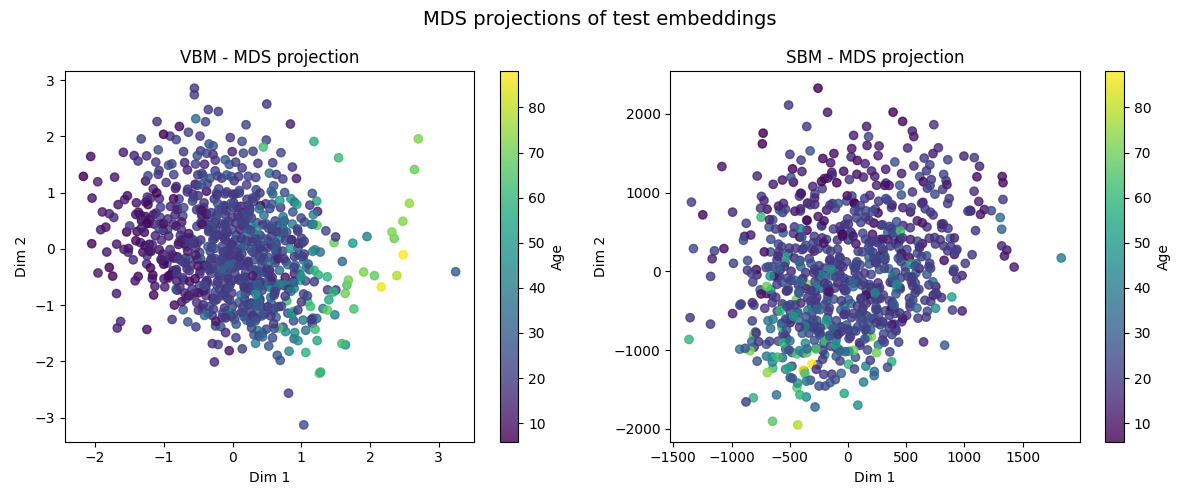
We then apply MDS on the test set and visualize the results. The points are colored according to the age of the subjects.
def plot_mds_side_by_side(Z_vbm, Z_sbm, y_vbm, y_sbm):
    """Run MDS on VBM and SBM embeddings and plot side-by-side scatter
    plots."""
    mds = MDS(n_components=2, n_init=4, max_iter=300)

    # Fit-transform embeddings
    Z_vbm_mds = mds.fit_transform(Z_vbm.cpu())
    Z_sbm_mds = mds.fit_transform(Z_sbm.cpu())

    # Side-by-side plots
    fig, axes = plt.subplots(1, 2, figsize=(12, 5))

    sc1 = axes[0].scatter(
        Z_vbm_mds[:, 0], Z_vbm_mds[:, 1], c=y_vbm, cmap="viridis", alpha=0.8
    )
    axes[0].set_title("VBM - MDS projection")
    axes[0].set_xlabel("Dim 1")
    axes[0].set_ylabel("Dim 2")
    plt.colorbar(sc1, ax=axes[0], label="Age")

    sc2 = axes[1].scatter(
        Z_sbm_mds[:, 0], Z_sbm_mds[:, 1], c=y_sbm, cmap="viridis", alpha=0.8
    )
    axes[1].set_title("SBM - MDS projection")
    axes[1].set_xlabel("Dim 1")
    axes[1].set_ylabel("Dim 2")
    plt.colorbar(sc2, ax=axes[1], label="Age")

    plt.suptitle("MDS projections of test embeddings", fontsize=14)
    plt.tight_layout()
    plt.show()


plot_mds_side_by_side(Z_test_vbm, Z_test_sbm, y_test_vbm, y_test_sbm)
Finally, we evaluate the learned representations on age prediction using linear regression and KNN regression. We report the mean absolute error and the R^2 coefficient between the true and predicted ages on the test set for each model.
def evaluate_and_predict(model, Z_train, Z_test, y_train, y_test):
    """Train model and return predictions + metrics."""
    model.fit(Z_train.cpu(), y_train)
    y_pred = model.predict(Z_test.cpu())
    mae = mean_absolute_error(y_test, y_pred)
    r2 = r2_score(y_test, y_pred)
    return y_pred, mae, r2


def plot_comparison(models, embeddings):
    """
    Plot side-by-side scatter plots for each model and modality.
    models: dict of {name: model}
    embeddings: dict of {modality: (Z_train, Z_test, y_train, y_test)}
    """
    n_models = len(models)
    n_modalities = len(embeddings)

    fig, axes = plt.subplots(
        n_models,
        n_modalities,
        figsize=(6 * n_modalities, 5 * n_models),
        sharex=True,
        sharey=True,
    )
    for row, (model_name, model) in enumerate(models.items()):
        for col, (modality, (Z_train, Z_test, y_train, y_test)) in enumerate(
            embeddings.items()
        ):
            y_pred, mae, r2 = evaluate_and_predict(
                model, Z_train, Z_test, y_train, y_test
            )

            ax = axes[row, col]
            ax.scatter(
                y_test,
                y_pred,
                alpha=0.7,
                color="orange" if modality == "SBM" else "steelblue",
            )
            ax.plot(
                [np.min(y_test), np.max(y_test)],
                [np.min(y_test), np.max(y_test)],
                "r--",
                lw=2,
                label="Ideal",
            )
            ax.set_title(
                f"{modality} - {model_name}\nMAE={mae:.2f}, R²={r2:.2f}"
            )
            ax.set_xlabel("True Age")
            if col == 0:
                ax.set_ylabel("Predicted Age")
            ax.legend()
            ax.grid(True)

    plt.suptitle("Model Comparison: VBM vs SBM", fontsize=16, y=1.02)
    plt.tight_layout()
    plt.show()


# Define models and embeddings
models = {
    "Linear Regression": LinearRegression(),
    "KNN (k=5)": KNeighborsRegressor(n_neighbors=5),
}

embeddings = {
    "VBM": (Z_train_vbm, Z_test_vbm, y_train_vbm, y_test_vbm),
    "SBM": (Z_train_sbm, Z_test_sbm, y_train_sbm, y_test_sbm),
}

# Run comparison
plot_comparison(models, embeddings)
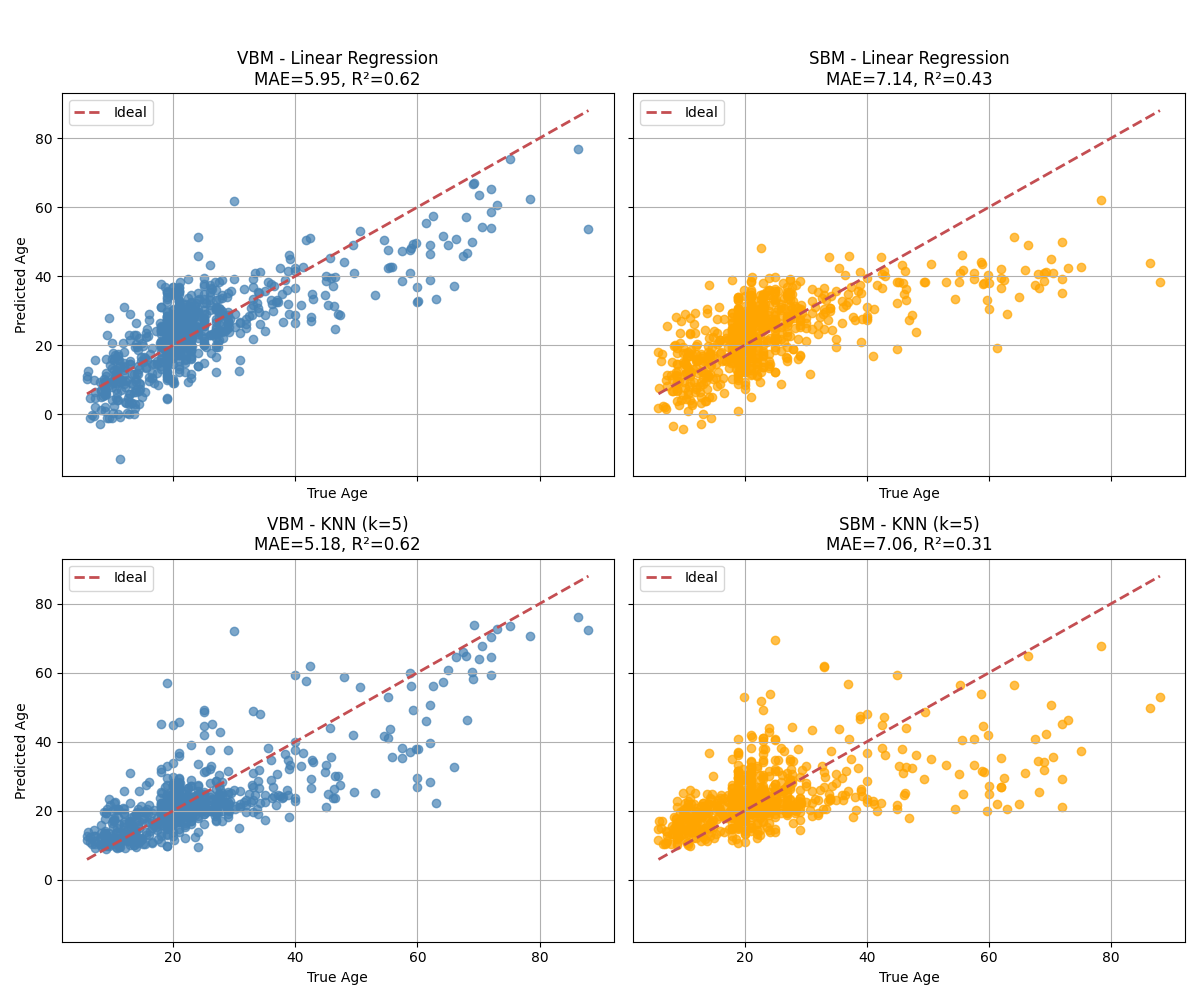
Observations: From the MDS visualizations, we can observe that both VBM and SBM embeddings show a gradient of ages, indicating that the models have learned to organize the data in a way that reflects age similarity. However, the VBM embeddings appear to have a more continuous distribution of ages compared to SBM. This suggests that VBM may capture age-related features more effectively than SBM in this context. This is confirmed when looking at the age prediction results, where VBM outperforms SBM for both linear regression and KNN regression. However, the results can be improved by working with the original 3d brain scans instead of the ROI-averaged data.
Total running time of the script: (6 minutes 50.573 seconds)
Estimated memory usage: 122 MB