Visualization of metrics during training of PyTorch-Lightning models

The current logic in nidl is to separate the implementation of the actual model (i.e. everything required to fit the model on data) from everything else, such as metrics computation and logging. This is usually performed to check the behavior of a model during training or validation but it is not essential for fitting.

This notebook will show you how to visualize some metrics (either given by torchmetrics, scikit-learn or a custom function score) during the training of a Pytorch Lightning model, using the MetricsCallback callback.

Setup

This notebook requires some packages besides nidl. Let’s first start with importing our standard libraries below:

import os
import re

import matplotlib.pyplot as plt
import torch.nn.functional as func
from tensorboard.backend.event_processing import event_accumulator
from torch import concat, nn
from torch.optim import SGD
from torch.utils.data import DataLoader
from torchmetrics import Accuracy, F1Score, Precision, Recall
from torchvision import transforms
from torchvision.datasets import MNIST
from torchvision.utils import make_grid

from nidl.callbacks import MetricsCallback
from nidl.estimators import BaseEstimator, ClassifierMixin
from nidl.estimators.ssl import SimCLR
from nidl.metrics.ssl import (
    alignment_score,
    contrastive_accuracy_score,
    uniformity_score,
)
from nidl.transforms import MultiViewsTransform

We define some global parameters that will be used throughout the notebook:

data_dir = "/tmp/mnist"
batch_size = 256
num_workers = 10
latent_size = 32

Classification metrics in supervised learning

For illustration purposes on how to use the metrics callback, we will focus on the popular MNIST dataset. It contains 60k training images and 10k test images of size 28x28 pixels. Each image contains a digit from 0 to 9. We will train a simple classification model on these data and log standard classification metrics (accuracy, F1-score, precision, recall) to understand how the MetricsCallback works.

We start by loading the MNIST dataset dataset with standard scaling transforms.

scale_transforms = transforms.Compose(
    [transforms.ToTensor(), transforms.Normalize((0.5,), (0.5,))]
)
train_xy_dataset = MNIST(data_dir, download=True, transform=scale_transforms)
test_xy_dataset = MNIST(
    data_dir, download=True, train=False, transform=scale_transforms
)

Then, we create the data loaders for training and testing the models.

train_xy_loader = DataLoader(
    train_xy_dataset,
    batch_size=batch_size,
    shuffle=True,
    drop_last=False,
    pin_memory=True,
    num_workers=num_workers,
)
test_xy_loader = DataLoader(
    test_xy_dataset,
    batch_size=batch_size,
    shuffle=False,
    drop_last=False,
    num_workers=num_workers,
)

/opt/hostedtoolcache/Python/3.12.12/x64/lib/python3.12/site-packages/torch/utils/data/dataloader.py:626: UserWarning: This DataLoader will create 10 worker processes in total. Our suggested max number of worker in current system is 4, which is smaller than what this DataLoader is going to create. Please be aware that excessive worker creation might get DataLoader running slow or even freeze, lower the worker number to avoid potential slowness/freeze if necessary.
  warnings.warn(

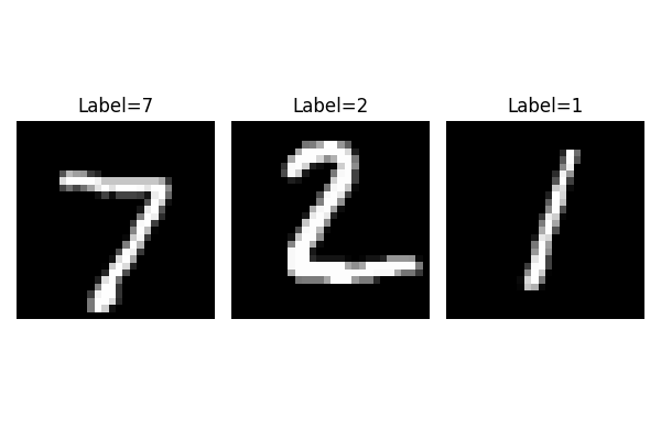
Before starting training classifiers, let’s visualize some examples of the dataset.

def show_images(images, title=None, nrow=8):
    grid = make_grid(images, nrow=nrow, normalize=True, pad_value=1)
    plt.figure(figsize=(10, 5))
    plt.imshow(grid.permute(1, 2, 0).cpu())
    if title:
        plt.title(title)
    plt.axis("off")
    plt.show()


images, labels = next(iter(test_xy_loader))
fig, axes = plt.subplots(1, 3, figsize=(6, 4))
for i in range(3):
    axes[i].imshow(images[i][0].cpu(), cmap="gray")
    axes[i].set_title(f"Label={labels[i].item()}")
    axes[i].axis("off")

plt.tight_layout()
plt.show()

Supervised training with metrics callback

Since MNIST images are small, we can use a simple LeNet-like architecture as encoder, with few parameters. The output dimension of the encoder is set to 32, which is approximately 30 times smaller that the input, but larger than the number of input classes (10).

class LeNet(nn.Module):
    def __init__(self, num_classes=10):
        super().__init__()
        self.latent_size = num_classes
        self.conv1 = nn.Conv2d(1, 6, kernel_size=5, stride=1, padding=2)
        self.pool1 = nn.AvgPool2d(2, 2)
        self.conv2 = nn.Conv2d(6, 16, kernel_size=5)
        self.pool2 = nn.AvgPool2d(2, 2)
        self.fc1 = nn.Linear(16 * 5 * 5, 120)
        self.fc2 = nn.Linear(120, 84)
        self.fc3 = nn.Linear(84, num_classes)

    def forward(self, x):
        x = func.relu(self.conv1(x))
        x = self.pool1(x)
        x = func.relu(self.conv2(x))
        x = self.pool2(x)
        x = x.view(x.size(0), -1)
        x = func.relu(self.fc1(x))
        x = func.relu(self.fc2(x))
        return self.fc3(x)

We can now fit a supervised model with cross-entopy loss (PL-compatible). We limit the training to 10 epochs for the sake of time and because it is enough for checking the evolution of the metrics across training.

class SupervisedCrossEntropy(ClassifierMixin, BaseEstimator):
    """Self-contained Pytorch-Lightning model.

    Metrics are not computed here since it is not essential to model's
    training.
    """

    def __init__(
        self,
        backbone: nn.Module,
        lr: float = 1e-2,
        momentum: float = 0.9,
        weight_decay: float = 5e-4,
        **kwargs,
    ):
        super().__init__(ignore=["callbacks", "backbone"], **kwargs)
        self.backbone = backbone
        self.lr = lr
        self.momentum = momentum
        self.weight_decay = weight_decay

    def configure_optimizers(self):
        optimizer = SGD(
            self.parameters(),
            lr=self.lr,
            momentum=self.momentum,
            weight_decay=self.weight_decay,
        )
        return [optimizer]

    def forward(self, imgs):
        return self.backbone(imgs)

    def training_step(
        self,
        batch,
        batch_idx: int,
        dataloader_idx: int = 0,
    ):
        imgs, labels = batch
        preds = self.backbone(imgs)
        loss = nn.functional.cross_entropy(preds, labels)
        self.log("loss/train", loss, on_step=True)
        return {
            "loss": loss,
            "preds": preds,
            "target": labels,
        }

    def validation_step(
        self,
        batch,
        batch_idx: int,
        dataloader_idx: int = 0,
    ):
        imgs, labels = batch
        preds = self.backbone(imgs)
        loss = nn.functional.cross_entropy(preds, labels)
        self.log("loss/val", loss, on_epoch=True)
        return {
            "val_loss": loss,
            "preds": preds,
            "target": labels,
        }

We create the metrics callback that will log the classification metrics during training every training step and every validation epoch (default):

callback = MetricsCallback(
    metrics={
        "acc1": Accuracy(task="multiclass", num_classes=10),
        "f1": F1Score(task="multiclass", num_classes=10),
        "precision": Precision(task="multiclass", num_classes=10),
        "recall": Recall(task="multiclass", num_classes=10),
    }
)

Finally, we fit the model:

model = SupervisedCrossEntropy(
    backbone=LeNet(),
    lr=1e-2,
    momentum=0.9,
    max_epochs=10,
    check_val_every_n_epoch=2,
    enable_checkpointing=False,
    callbacks=callback,  # <-- key part for metrics computation
)
model.fit(train_xy_loader, test_xy_loader)

┏━━━┳━━━━━━━━━━┳━━━━━━━┳━━━━━━━━┳━━━━━━━┳━━━━━━━┓
┃   ┃ Name     ┃ Type  ┃ Params ┃ Mode  ┃ FLOPs ┃
┡━━━╇━━━━━━━━━━╇━━━━━━━╇━━━━━━━━╇━━━━━━━╇━━━━━━━┩
│ 0 │ backbone │ LeNet │ 61.7 K │ train │     0 │
└───┴──────────┴───────┴────────┴───────┴───────┘
Trainable params: 61.7 K
Non-trainable params: 0
Total params: 61.7 K
Total estimated model params size (MB): 0
Modules in train mode: 8
Modules in eval mode: 0
Total FLOPs: 0
/opt/hostedtoolcache/Python/3.12.12/x64/lib/python3.12/site-packages/torch/utils/data/dataloader.py:665: UserWarning: 'pin_memory' argument is set as true but no accelerator is found, then device pinned memory won't be used.
  warnings.warn(warn_msg)
Epoch 9/9  ━━━━━━━━━━━━━━━━ 235/235 0:00:09 •        27.63it/s v_num: 8.000
                                    0:00:00                    acc1/train: 0.990
                                                               f1/train: 0.990
                                                               precision/train:
                                                               0.990
                                                               recall/train:
                                                               0.990 acc1/val:
                                                               0.977 f1/val:
                                                               0.977
                                                               precision/val:
                                                               0.977 recall/val:
                                                               0.977

SupervisedCrossEntropy(
  (backbone): LeNet(
    (conv1): Conv2d(1, 6, kernel_size=(5, 5), stride=(1, 1), padding=(2, 2))
    (pool1): AvgPool2d(kernel_size=2, stride=2, padding=0)
    (conv2): Conv2d(6, 16, kernel_size=(5, 5), stride=(1, 1))
    (pool2): AvgPool2d(kernel_size=2, stride=2, padding=0)
    (fc1): Linear(in_features=400, out_features=120, bias=True)
    (fc2): Linear(in_features=120, out_features=84, bias=True)
    (fc3): Linear(in_features=84, out_features=10, bias=True)
  )
)

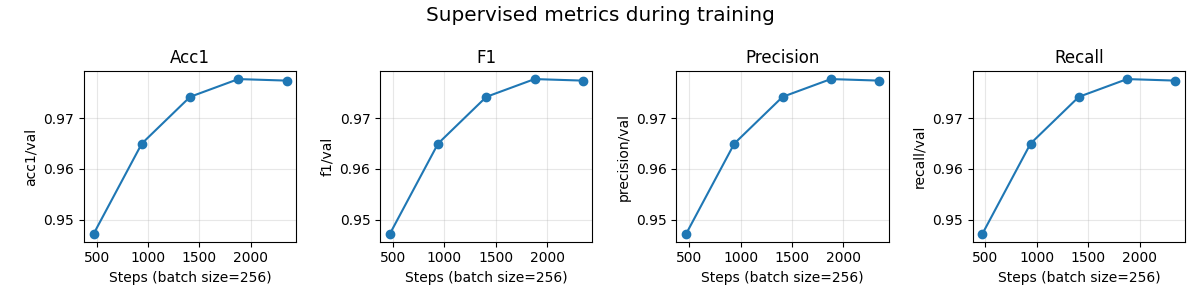
Visualization of the classification metrics during training

During training, we can visualize the classification metrics logged by the MetricsCallback using TensorBoard. The logged metrics are stored in the lightning_logs folder by default. They contain the accuracy, F1-score, precision (macro) and recall (macro).

def get_last_log_version(logs_dir="lightning_logs"):
    versions = []
    for d in os.listdir(logs_dir):
        match = re.match(r"version_(\d+)", d)
        if match:
            versions.append(int(match.group(1)))
    return max(versions) if versions else None


log_dir = f"lightning_logs/version_{get_last_log_version()}/"
ea = event_accumulator.EventAccumulator(log_dir)
ea.Reload()
metrics = [
    "acc1/val",
    "f1/val",
    "precision/val",
    "recall/val",
]
scalars = {m: ea.Scalars(m) for m in metrics}

Once all the metrics are loaded, we plot them as the number of training steps increases:

num_metrics = len(scalars)
fig, axes = plt.subplots(1, num_metrics, figsize=(3 * num_metrics, 3))

for ax, (metric_name, events) in zip(axes, scalars.items()):
    steps = [e.step for e in events]
    values = [e.value for e in events]

    ax.plot(steps, values, marker="o", linestyle="-")
    ax.set_title(metric_name.split("/")[0].capitalize())
    ax.set_xlabel(f"Steps (batch size={batch_size})")
    ax.set_ylabel(metric_name)
    ax.grid(True, alpha=0.3)

plt.suptitle("Supervised metrics during training", fontsize="x-large")
plt.tight_layout()
plt.show()

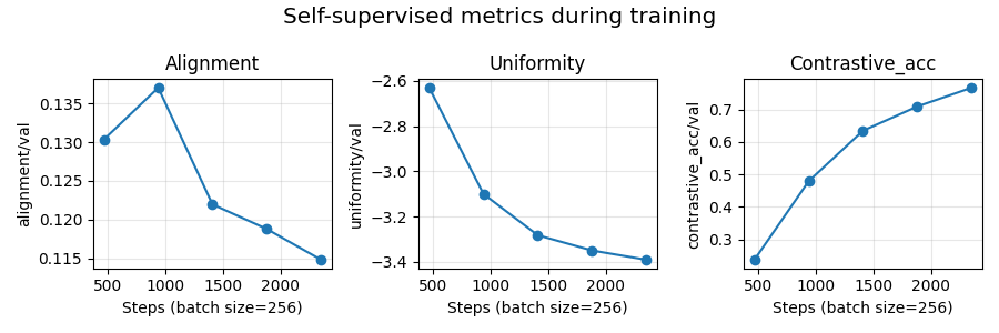
Unsupervised contrastive learning with metrics callback

We now demonstrate how to plot self-supervised metrics (alignment and uniformity scores) during the training of a SimCLR model (implementation from NIDL). The logic is the same as before.

Dataset and data augmentations for contrastive learning

To perform self-supervisde contrastive learning, we need to define a set of data augmentations to create multiple views of the same image. Since we work with grayscale images, we will use random resized crop and Gaussian blur. We reduce the size of the Gaussian kernel to 3x3 since MNIST images are only 28x28 pixels.

contrast_transforms = transforms.Compose(
    [
        transforms.RandomResizedCrop(size=28, scale=(0.8, 1.0)),
        transforms.GaussianBlur(kernel_size=3),
        transforms.ToTensor(),
        transforms.Normalize((0.5,), (0.5,)),
    ]
)

We create a MNIST dataset that returns multiple views of the same image.

ssl_dataset = MNIST(
    data_dir,
    download=True,
    transform=MultiViewsTransform(contrast_transforms, n_views=2),
)
test_ssl_dataset = MNIST(
    data_dir,
    download=True,
    train=False,
    transform=MultiViewsTransform(contrast_transforms, n_views=2),
)

train_ssl_loader = DataLoader(
    ssl_dataset,
    batch_size=batch_size,
    shuffle=True,
    pin_memory=True,
    num_workers=num_workers,
)
test_ssl_loader = DataLoader(
    test_ssl_dataset,
    batch_size=batch_size,
    shuffle=False,
    pin_memory=True,
    num_workers=num_workers,
)

Now, we create the callback that will compute and log the self-supervised metrics during training and validation.

Important remark: uniformity score cannot be aggregated with a simple average over batch as the alignment score. Here, we perform an exact computation of the uniformity score on the validation set only. The score on the training set is just an approximation but we don’t require exact computation as the model’s weights are changing over iterations.

callback = MetricsCallback(
    metrics={
        "alignment": alignment_score,
        "uniformity": uniformity_score,
        "contrastive_acc": contrastive_accuracy_score,
    },
    needs={
        "alignment": ["z1", "z2"],
        "uniformity": {"z": lambda out: concat((out["z1"], out["z2"]))},
        "contrastive_acc": ["z1", "z2"],
    },
    every_n_train_steps=None,
    every_n_val_epochs=2,
)

model = SimCLR(
    encoder=LeNet(num_classes=latent_size),
    proj_input_dim=latent_size,
    proj_hidden_dim=latent_size,
    proj_output_dim=32,
    learning_rate=3e-4,
    temperature=0.1,
    weight_decay=5e-5,
    max_epochs=10,
    enable_checkpointing=False,
    callbacks=callback,  # <-- key part for metrics computation
)

model.fit(train_ssl_loader, test_ssl_loader)

┏━━━┳━━━━━━━━━━━━━━━━━┳━━━━━━━━━━━━━━━━━━━━━━┳━━━━━━━━┳━━━━━━━┳━━━━━━━┓
┃   ┃ Name            ┃ Type                 ┃ Params ┃ Mode  ┃ FLOPs ┃
┡━━━╇━━━━━━━━━━━━━━━━━╇━━━━━━━━━━━━━━━━━━━━━━╇━━━━━━━━╇━━━━━━━╇━━━━━━━┩
│ 0 │ encoder         │ LeNet                │ 63.6 K │ train │     0 │
│ 1 │ projection_head │ SimCLRProjectionHead │  2.1 K │ train │     0 │
│ 2 │ loss            │ InfoNCE              │      0 │ train │     0 │
└───┴─────────────────┴──────────────────────┴────────┴───────┴───────┘
Trainable params: 65.7 K
Non-trainable params: 0
Total params: 65.7 K
Total estimated model params size (MB): 0
Modules in train mode: 14
Modules in eval mode: 0
Total FLOPs: 0
Epoch 9/9  ━━━━━━━━━━━━━━━━ 235/235 0:00:44 • 0:00:00 5.71it/s v_num: 9.000
                                                               loss/train: 0.315
                                                               loss/val: 1.139
                                                               alignment/val:
                                                               0.115
                                                               uniformity/val:
                                                               -3.390
                                                               contrastive_acc/…
                                                               0.766

SimCLR(
  (encoder): LeNet(
    (conv1): Conv2d(1, 6, kernel_size=(5, 5), stride=(1, 1), padding=(2, 2))
    (pool1): AvgPool2d(kernel_size=2, stride=2, padding=0)
    (conv2): Conv2d(6, 16, kernel_size=(5, 5), stride=(1, 1))
    (pool2): AvgPool2d(kernel_size=2, stride=2, padding=0)
    (fc1): Linear(in_features=400, out_features=120, bias=True)
    (fc2): Linear(in_features=120, out_features=84, bias=True)
    (fc3): Linear(in_features=84, out_features=32, bias=True)
  )
  (projection_head): SimCLRProjectionHead(
    (layers): Sequential(
      (0): Linear(in_features=32, out_features=32, bias=True)
      (1): ReLU()
      (2): Linear(in_features=32, out_features=32, bias=True)
    )
  )
  (loss): InfoNCE(temperature=0.1)
)

Visualization of the self-supervised metrics during training

As before, we visualize the logged metrics using tensorboard.

def get_last_log_version(logs_dir="lightning_logs"):
    versions = []
    for d in os.listdir(logs_dir):
        match = re.match(r"version_(\d+)", d)
        if match:
            versions.append(int(match.group(1)))
    return max(versions) if versions else None


log_dir = f"lightning_logs/version_{get_last_log_version()}/"
ea = event_accumulator.EventAccumulator(log_dir)
ea.Reload()
metrics = ["alignment/val", "uniformity/val", "contrastive_acc/val"]
scalars = {m: ea.Scalars(m) for m in metrics}

Once all the metrics are loaded, we plot them as the number of training steps increases:

num_metrics = len(scalars)
fig, axes = plt.subplots(1, num_metrics, figsize=(3 * num_metrics, 3))

for ax, (metric_name, events) in zip(axes, scalars.items()):
    steps = [e.step for e in events]
    values = [e.value for e in events]

    ax.plot(steps, values, marker="o", linestyle="-")
    ax.set_title(metric_name.split("/")[0].capitalize())
    ax.set_xlabel(f"Steps (batch size={batch_size})")
    ax.set_ylabel(metric_name)
    ax.grid(True, alpha=0.3)

plt.suptitle("Self-supervised metrics during training", fontsize="x-large")
plt.tight_layout()
plt.show()

Estimated memory usage: 2402 MB